Dead time, live time and real time

Definition

Real time is the time during which a measurement is performed.

Dead time is defined as the period of time during which data cannot be collected or has been locked. Whenever a gamma particle is absorbed by the scintillation crystal, the crystal absorbs its energy and re-emits the absorbed energy in the form of light. The light pulse is processed and analyzed by the system. Until the light pulse has died out and the signal has been processed, the system will not register any new gamma particles. The dead time depends on the count rate, the type of scintillation crystal and the electronics.

Live time is the time during which the spectrometer was actually "open" to data. Live time can be calculated using:

t_l = t_r - t_d

Where t_l, t_r and t_d are live time, real time and dead time.

Converting measured counts c_m into real counts c_r involves:

c_r = c_m * t_r / t_l = c_m * t_r / (t_r - t_d)

Example: Suppose we have measured 1000 counts over a period of exactly 1 second (the real time, t_r). The dead time t_d during this measurement was 0.01 seconds. This would mean the live time t_l is 1.00 - 0.01 = 0.99 seconds. Effectively, we have registered 1000 counts not in 1 second, but in 0.99 seconds. This means the count rate is 1000 / 0.99 = 1010.1 counts per second! As dead time increases with count rate, this effect may become significant at large count rates.

Calculation of dead time

Calculation of the dead time is often done by the hardware. There are different approaches to calculating the dead time.

Using a fast counter

One option is to include a fast counter, which registers all gamma events, but doesn't analyze them. The dead time is then calculated using:

t_d = t_r * (c_m - c_f) / c_f

Where c_m is the number of counts registered in the spectrum and c_f is the number of counts registered by the fast counter.

In the example above, during the 1 seconds of real time, the spectrum will hold 1000 counts, while the fast counter may have registered 1010 counts, leading to a dead time of 1 * (1010 - 1000) / 1010 = 0.01 seconds.

Using a fixed dead time per count

This approach is very simple, as it assumes a fixed dead time τ for each registered count. Typically, τ is around 5 microseconds. For low count rates, the dead time can be calculated using:

t_d = τ * c_m

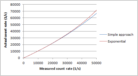
Since it is possible for new gamma particles to be absorbed by the scintillation crystal during a period of dead time, the dead time can be extended, and it would be better to use:

t_d = 1 - exp(-τ * c_r)    where c_r can be calculated from    c_m = c_r * exp(-τ * c_r)

The latter formula can only be solved numerically, so the first equation is often used instead. The figure below shows the first equation gives a very good approximation for low count rates (graph depending on the deadtime per count, of course):

Measuring τ

There are several approaches for measuring the dead time per count τ. All methods discussed below involve the measurement of a count rate R, using 1 or 2 radioactive sources. All methods require proper background correction (perform a measurement without the source, and subtract the background count rate from all other measurements).

1. Using a rapid decaying source

This approach requires the use of a rapid decaying point source in a fixed position. The source should decay at a well known rate (either decay in a single process or having reached a stable situation). Sources which can be used in this approach have a half life of a few hours to a few days. Suitable sources which are also used in nuclear medicine include jodium-123 and technetium-99m. Using the known decay constant λ for the source, it is possible to predict the count rate at a certain time t:

R_r(t) = R_r(0) * exp(-λ * t)

Where R_r(t) is the real count rate at time t.

The measured count rate R_m relates to the real count rate R_r through:

R_r(t) = R_m(t) / (1 - R_m(t) * τ)

Combining both equations gives:

R_r(0) = R_m(t) / (1 - R_m(t) * τ) * exp(λ * t)

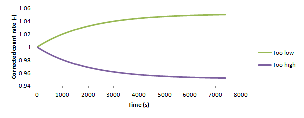
The last equation should give a constant value for R_r(0), for all values of t. Using a series of measurements and a best fit approach (using for example MS Excel), this should give a value of τ which best describes the dead time per count in the system.

The figure below shows effects of values for τ which are too high or too low:

2. Using a point source at different positions

When using a point source with 'constant' activity (the half-life should be relatively large, preferably at least a few years), it is possible to determine τ by changing the distance d between source and detector. In this case, the count rate can be calculated using:

R_r(0) ~ R_r(d) * d²

This results in an equation

R_r(0) ~ R_m(t) / (1 - R_m(t) * τ) * d²

The last equation should give a constant value for R_r(0), for all values of d. Using a series of measurements and a best fit approach (using for example MS Excel), this should give a value of τ which best describes the dead time per count in the system

Note that this method assumes a point source and an infinitely small detector. For values of d which are large enough, this method may still yield a good approximation of τ.

3. Using 2 point sources

The method involves the use of 2 point sources and uses the equation:

R_r = R_m / (1 - R_m * τ)

If we denote the real count rate from source 1 as R_r,1 that of source 2 as R_r,2, and that of both sources combined as R_r,1+2 we can write: 

R_r,1 = R_m,1 / (1 - R_m,1 * τ),       R_r,2 = R_m,2 / (1 - R_m,2 * τ)        and        R_r,1+2 = R_m,1+2 / (1 - R_m,1+2 * τ) 

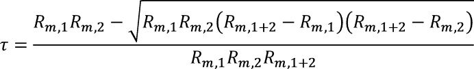
Rewriting to exclude all real count rates R_r results in: